
 Module 4
Designing a Vector Search System
You know the primitives. This module is about judgment: how to go from “I have data and users” to a concrete design, making the same decisions you’d make on a real project.
Today’s path
- The Layers of the Stack
- Worked Example: Designing a Multilingual News Search System
- Filtering, Properly
- The Production RAG Pipeline
- Deployment Options
- Knowledge Check
- References & Further Reading
By the end, you’ll be able to reason about any vector search architecture layer by layer, and you’ll have designed one system end to end.
1. The Layers of the Stack
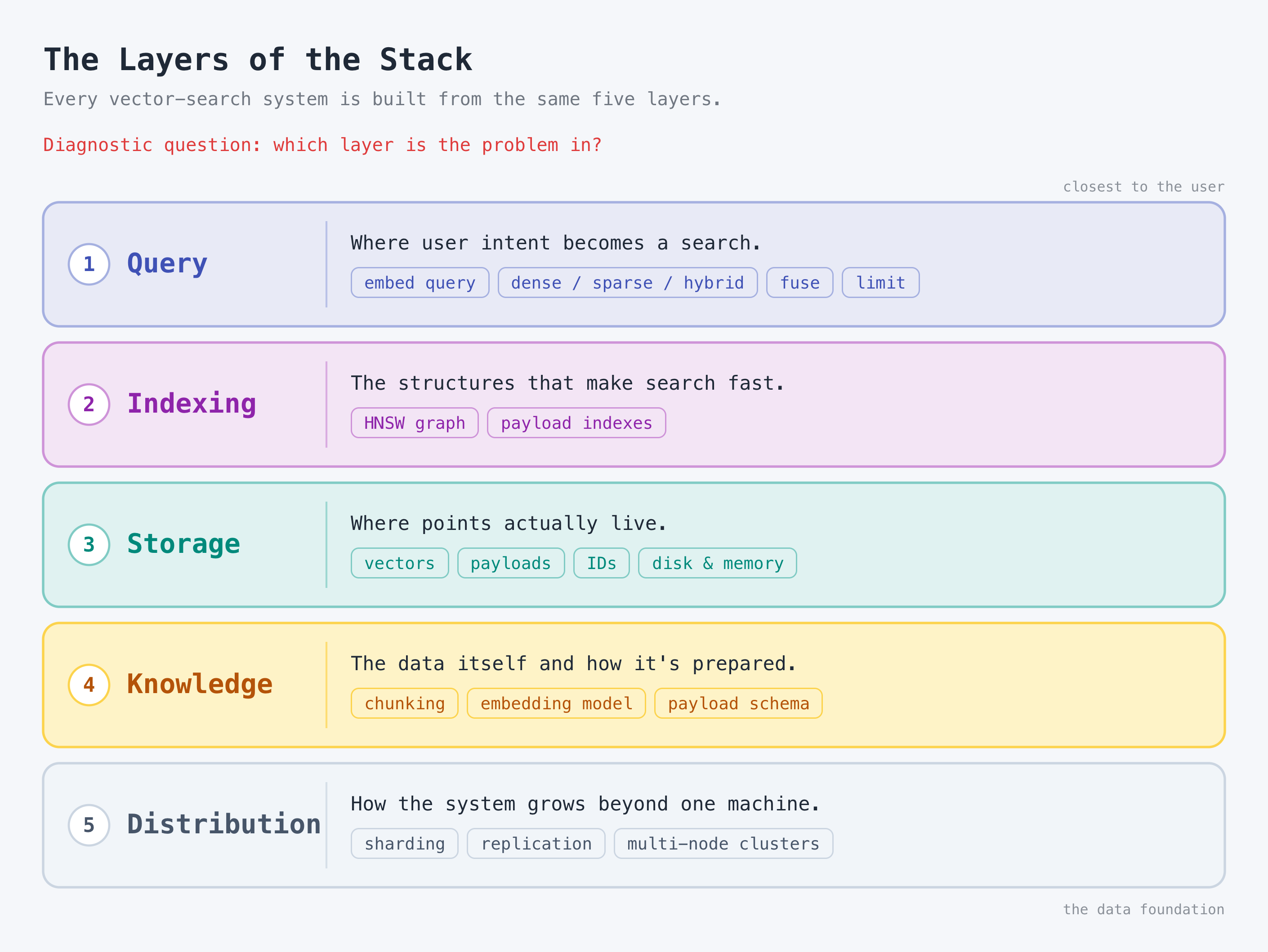
Every vector search system, from a notebook prototype to a deployment serving millions of queries, is built from the same five layers. When something is slow, wrong, or expensive, the first diagnostic question is always the same: which layer is the problem in?
- Query layer: Where user intent becomes a search. Embedding the query, choosing dense vs. sparse vs. hybrid, fusing results, setting limits. This is the layer you worked in throughout Module 3.
- Indexing layer: The structures that make search fast: the HNSW graph for vectors (Module 2) and payload indexes for filter fields. Mistakes here don’t make results wrong. They make everything slow.
- Storage layer: Where points actually live: vectors, payloads, and IDs on disk and in memory. Decisions about what goes in each point’s payload, and how big your vectors are, land here.
- Knowledge layer: The data itself and how it’s prepared: chunking, embedding model choice, payload schema design. Problems in this layer can’t be fixed by tuning any other layer. Garbage in, garbage retrieved.
- Distribution layer: How the system grows beyond one machine: sharding, replication, multi-node clusters. You don’t need this on day one. Growing systems eventually do.
Key insight
Every design decision belongs to a layer. “Add a payload index” is an indexing decision. “Switch to a multilingual embedding model” is a knowledge decision. “Move to three nodes” is a distribution decision. Once you sort decisions into layers, intimidating architecture diagrams become checklists.
2. Worked Example: Designing a Multilingual News Search System
Rather than reading about someone else’s architecture, let’s design one. The brief:
Analysts at a research firm need to search global news. Articles arrive continuously in many languages. Analysts ask questions in English (“port congestion in Southeast Asia”), expect results from any language, and need to scope searches by country, topic, date range, and source. Some queries name exact things, like a company ticker or a ship name, that must match precisely.
That’s realistic, and it’s messy in exactly the ways real projects are. We’ll design it by answering five questions. Each answer is a decision in a specific layer.
Question 1: What’s the workload shape?
How much data, in what modalities, arriving how fast?
Millions of articles, text-only for now, arriving continuously. Hundreds of thousands of new chunks per day, and analysts expect this morning’s news to be searchable this morning.
Decisions: one collection; continuous upserts rather than batch rebuilds (Qdrant indexes as it ingests, so there’s nothing to design around); plan the payload schema now, because re-ingesting millions of articles later is painful. (Storage and knowledge layers.)
Question 2: What do the queries look like?
Natural language? Exact tokens? Both?
Both, and this is the single most consequential observation in the whole design. “Port congestion in Southeast Asia” is semantic intent: dense territory. “MAERSK-B.CO delisting” is an exact token that dense search will happily blur into neighboring tickers. You saw this failure in Module 3 as the SKU problem.
Decision: hybrid from the start. Named dense and sparse vectors on every point, RRF fusion at query time. (Query layer.)
from qdrant_client import QdrantClient, models

client = QdrantClient(url=..., api_key=...)

client.create_collection(
    collection_name="news",
    vectors_config={
        "dense": models.VectorParams(size=1024, distance=models.Distance.COSINE),
    },
    sparse_vectors_config={
        "sparse": models.SparseVectorParams(),
    },
)
Question 3: What must the system filter on?
Which constraints are hard rules, not similarity signals?
From the brief: country, topic, date range, and source. These aren’t “nice to rank higher” signals. An analyst scoping to “Vietnam, last 7 days” means exactly that. Hard rules go in the payload; Section 3 covers why this works at speed.
Decision: the payload schema, designed now, before ingestion:
payload:
  country       string    (indexed)
  language      string    (indexed)
  topic         string    (indexed)
  source        string    (indexed)
  published_at  datetime  (indexed)
  summary       string    (not indexed: returned, never filtered)
(Knowledge and indexing layers.)
Question 4: What does the retrieval pipeline look like?
Dense-only? Hybrid? Reranking?
Start with the simplest pipeline that fits the query analysis: hybrid (from Question 2) plus filters (from Question 3), fused with RRF. No reranker yet. Add one only if evaluation shows fused results need refinement. Complexity is added when data proves it’s needed, never in advance.
One knowledge-layer decision hides in here: the embedding model must be multilingual. Analysts query in English but articles arrive in Japanese, Vietnamese, and Mandarin. A multilingual model projects all languages into one vector space, so an English query retrieves a Japanese article with no translation step. A monolingual English model makes cross-language retrieval structurally impossible, and no amount of query-layer tuning fixes a knowledge-layer mistake.
results = client.query_points(
    collection_name="news",
    prefetch=[
        models.Prefetch(query=dense_vec,  using="dense",  limit=50),
        models.Prefetch(query=sparse_vec, using="sparse", limit=50),
    ],
    query=models.FusionQuery(fusion=models.Fusion.RRF),
    query_filter=models.Filter(
        must=[
            models.FieldCondition(key="country", match=models.MatchValue(value="VN")),
            models.FieldCondition(key="published_at",
                                  range=models.Range(gte="2026-07-01T00:00:00Z")),
        ]
    ),
    limit=10,
)
(Query layer, with one knowledge-layer dependency.)
Question 5: What are the deployment constraints?
Latency budget, data residency, cost, and who operates this thing?
A research firm with a small engineering team, no residency restrictions, and a “please don’t page us at night” operational budget points to a managed deployment. The same design would run self-hosted if the constraints said otherwise. The design and the deployment mode are independent decisions; Section 5 lays out the full option space. (Distribution layer.)
The Design on One Page
| Question | Answer for this system | Layer |
|---|---|---|
| Workload shape | Millions of text chunks, continuous ingestion | Storage, knowledge |
| Query type | Mixed semantic + exact, so hybrid with RRF | Query |
| Filter scope | country, topic, source, date in an indexed payload | Knowledge, indexing |
| Pipeline | Hybrid + filters; multilingual model; no reranker yet | Query, knowledge |
| Deployment | Managed; design independent of the choice | Distribution |
Key insight
Nothing in this design is exotic. It’s the Module 2 pipeline plus the Module 3 hybrid pattern plus a payload schema that was thought about before ingestion. That last part is what separates systems that scale from systems that get re-ingested three times. Use the five questions on any system you’re asked to design, including the one you’ll build in Module 5.
3. Filtering, Properly
Filters showed up in every module so far: a must condition here, a date range there. Time to treat filtering as what it is in production: the feature that decides whether your results are correct, not an accessory to similarity.
Why Filtering During Traversal Matters
There are two ways to combine filters with vector search.
- Post-filtering (the naive way): Retrieve top-K by similarity, then discard results that fail the filter. The problem: with a selective filter, say one country out of two hundred or one week out of a decade of archives, the top-K may contain zero valid results. Retrieving a bigger K to compensate gets slow fast, and there’s no K that guarantees correctness.
- Filtered traversal: The filter is applied while walking the HNSW graph. Invalid points never enter the candidate set, so results are both semantically relevant and guaranteed valid, at speed. This is how Qdrant applies
query_filter, and it’s why filtering on every query is a safe default rather than a performance concern.
The Filter Toolbox
| Condition | Logic | Example from the news system |
|---|---|---|
| must | AND: all conditions true | country = VN AND topic = shipping |
| should | OR: at least one true | topic = shipping OR topic = logistics |
| must_not | Exclude matches | Exclude source = press-release wire |
| Range | Numeric or datetime bounds | published_at within the last 7 days |
| Geo | Radius or bounding box | Events within 100 km of a port |
| MatchAny | Value in a set | language in [“ja”, “zh”, “ko”] |
| Nested | Conditions inside array payloads | Any mention with company = X AND sentiment < 0 |
Conditions compose. A realistic analyst query combines must (country), Range (recency), MatchAny (languages), and must_not (excluded sources) in one filter, evaluated together during traversal.
Index What You Filter
Without a payload index, Qdrant scans every payload at query time: O(n). With one, filtered queries run in logarithmic time. The rule: every field that appears in must, should, or must_not gets an index, with a schema type matching the data.
for field in ["country", "language", "topic", "source"]:
    client.create_payload_index(
        collection_name="news",
        field_name=field,
        field_schema=models.PayloadSchemaType.KEYWORD,
    )

client.create_payload_index(
    collection_name="news",
    field_name="published_at",
    field_schema=models.PayloadSchemaType.DATETIME,
)
Schema types: KEYWORD for exact strings, INTEGER and FLOAT for numbers, DATETIME for timestamps, GEO for coordinates, TEXT for full-text conditions.
A Special Case Worth Knowing: Scoping by User or Tenant
One filtering pattern deserves a call-out because you’ll meet it in almost any multi-user product: scoping every query to one user’s (or one customer’s) data. The instinct is to create a collection per user. With many users, that becomes thousands or millions of collections, which is operationally unmanageable. The standard pattern instead:
- Add a
tenant_id(oruser_id) payload field to every point at ingestion. - Create a payload index on it.
- Filter on it at every query. Never omit it.
One collection, complete per-tenant isolation at query time, and thanks to filtered traversal plus the index, it stays fast at any tenant count. This is the same mechanism as the country filter in the news system, just applied to identity instead of geography. See Multitenancy - Qdrant for the full pattern, including how to combine it with Qdrant’s tenant-aware HNSW optimizations.
Key insight
Design the payload schema before you ingest, driven by one question: what will I need to filter on? Time, geography, identity, permissions, and status flags are the usual suspects. Adding a payload field later is easy. Discovering at query time that you never stored language is not.
4. The Production RAG Pipeline
Retrieval-Augmented Generation (RAG) is the pattern of retrieving relevant passages from a vector database and handing them to an LLM as context, so the model answers from your data instead of relying only on what it memorized during training. If the news system grows an “ask a question, get an answer with sources” feature, it becomes a RAG pipeline - the most common architecture built on vector search today. The production shape, using everything covered so far:
- Query understanding: Extract hard constraints from the request (dates, country, topic) into a filter. Embed the query as a dense vector and a sparse vector.
- Hybrid retrieval:
Prefetch(dense, filter, limit=50)+Prefetch(sparse, filter, limit=50), thenFusionQuery(RRF), returning the top 20 candidates. Onequery_pointscall. - Optional reranking: A cross-encoder scores the top 20 and keeps the top 5. Add this stage only when evaluation shows fused results need refinement.
- LLM generation: The top-k passages go in as context; the model generates the answer.
Rule of thumb
When RAG quality disappoints, improve step 2 before reaching for a bigger model in step 4. Retrieval quality caps answer quality: the model can’t cite a passage it never received.
Beyond RRF, Qdrant also supports payload-aware scoring, like boosting recent articles over stale ones or demoting items a user already dismissed, via formula queries. You won’t need them for the capstone; the course’s closing video points you there as a further-learning topic.
5. Deployment Options
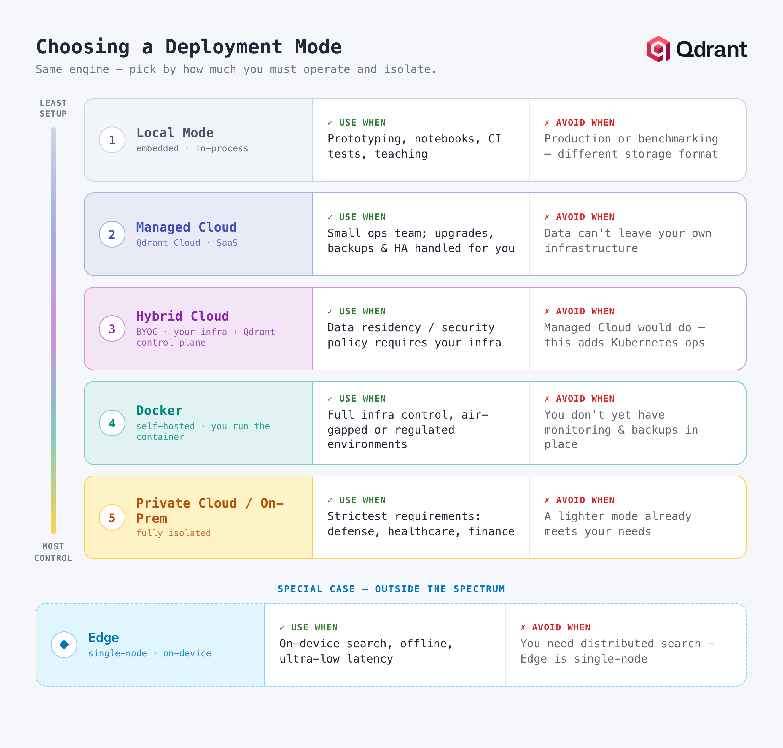
The news system’s design runs unchanged on any deployment mode. Which one is right depends on constraints, not sophistication.
| Deployment Mode | Use When | Avoid When |
|---|---|---|
| Local Mode | Prototyping, notebooks, CI tests, teaching | Production or benchmarking (different storage format) |
| Docker (Self-Hosted) | Full infra control, air-gapped, regulated environments | You don’t yet have monitoring and backups in place |
| Managed Cloud | Small ops team, standard requirements: upgrades, backups, HA handled for you | Data can’t leave your infrastructure |
| Hybrid Cloud (BYOC) | Data residency or security policy requires your infrastructure | Managed cloud would do; this adds Kubernetes ops complexity |
| Private Cloud / On-Prem | Strictest requirements: defense, healthcare, finance | A lighter mode meets your needs |
| Edge | On-device search, offline, ultra-low latency | You need distributed search (Edge is single-node) |
6. Knowledge Check
Work through these before starting the capstone.
Q: Name the five layers of a vector search stack, and place “switch to a multilingual embedding model” in the right one.
A: Query, indexing, storage, knowledge, distribution. The embedding model is a knowledge-layer decision, and mistakes there can’t be fixed by tuning other layers.
Q: In the news system, why is hybrid retrieval chosen from the start rather than dense-only?
A: Query analysis showed a mix of semantic intent (“port congestion”) and exact tokens (tickers, ship names). Dense search blurs exact tokens into semantic neighbors, the SKU problem from Module 3, so a sparse vector is needed alongside dense, fused with RRF.
Q: What’s the difference between post-filtering and filtered traversal, and why does it matter for selective filters?
A: Post-filtering retrieves top-K first and discards invalid results; with a selective filter, the top-K may contain zero valid points. Filtered traversal applies conditions while walking the HNSW graph, so invalid points never enter the candidate set.
Q: Why does per-user scoping use a payload filter instead of one collection per user?
A: Collections don’t scale to millions of users operationally. An indexed tenant_id payload field, filtered on at every query, gives complete isolation in one collection at full speed. It’s the same mechanism as any other keyword filter.
Q: In the RAG pipeline, which step should you improve first when answer quality disappoints, and why?
A: Step 2, retrieval. Retrieval quality caps answer quality, since the model can’t cite a passage it never received. Improving the retriever beats scaling the LLM.
Q: When would you choose Hybrid Cloud over managed cloud, and when would you not?
A: Choose it when data residency or security policy requires your own infrastructure. Otherwise skip it: it adds Kubernetes operational complexity you don’t need.
7. References & Further Reading
Filtering Reference - Filtering - Qdrant
- Full filter syntax: must, should, must_not, range, geo, and nested conditions.
Payload Indexes - Indexing - Qdrant
- Keyword, datetime, float, and geo payload index configuration.
Multi-Tenancy Guide - Multiple Partitions - Qdrant
- The payload-based tenant scoping pattern in depth.
Hybrid Search Tutorial - Hybrid Search with FastEmbed - Qdrant
- Dense + sparse with FastEmbed and RRF fusion, step by step.
Deployment Documentation - Qdrant Cloud - Qdrant
- All deployment modes with configuration references.
What’s Next - Module 5
Next, the capstone extends the system you just designed. Same design questions, bigger answers:
- Ingest daily news, audio, and satellite imagery about suppliers: three modalities instead of one
- Embed each modality into named vectors on shared points
- Cluster signals into risk themes across suppliers
- Query across languages: ask in English, retrieve Japanese and Chinese sources
End of Module 4. Continue to Module 5: the hands-on capstone project.